Contents

• 1. Data Preparation
  • 1) Reading and Cleaning Data
  • 2) Principal Component Analysis (PCA)
  • 3) Cross-check
  • 4) Custom Functions
• 2. Dog Breed Classification Models
  • 1) K-Nearest Neighbors (Varying Image Size)
  • 3) AdaBoost Classification
  • 4) Decision Tree Classification
  • 5) Random Forest Classification
  • 6) Mixture of Classifiers Classification (Ensembling)
• 3. Conclusion & Future Work

1. Data Preparation

1) Reading and Cleaning Data

In order to classify dog breeds, we leveraged the various models taught from class material. However, before perfoming classifications on each model, we had to first preprocess our input data. Our group quickly discovered that the image files imported all suffered noise distortion and irregular image dimensions. Thus to unify our photos, our team assigned a bounding box region to eliminate redundant background features, then cropped each photo such that solely the dog in question was visible.

We then resized each image to a unified dimension specified by the user. As the unified image size was a variable subject to the user’s discretion, we opted to run our classification models iteratevly in order to obtain the best model accuracy (in respect to universal image size).

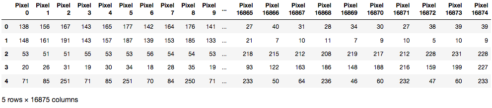
We then finalized our data preparation process by generating a list of pixel features, storing each image pixel list into a corresponding dataframe. We obtain this list of pixel features by first flattening each image’s multi-dimensional pixel array, and return the associated single dimensional dataset.

# The desired image output size, this will unify all images to this size
size = 75

# Obtain the pixel matrix and classification list from the requested images
imgPixMat, imgClassMat = load_images_from_folder('./Dog Images/n02096585-Boston_bull', './Annotation/n02096585-Boston_bull/', size)

# Generate column names for every pixel in our matrix
columnNames = []

# Note: the range is for a flattened pixel vector, therefore an image of size N has N Squared Red, Blue, Green pixels
# .. Simply multiplying N Squared by 3 gets us our total pixel count for the image. 
for i in range(0, (np.power(size,2)*3)):
    columnNames.append(('Pixel '+str(i)))

# Create a dataframe to store all pixel values
data_df = pd.DataFrame(columns=columnNames)

# Append our pixel values to the dataframe
data_df = DfAppend_Vals(data_df, imgPixMat, columnNames)

data_df.head()

# Create a dataframe to store all classification values
class_df = pd.DataFrame(columns=['Class'])

class_df = DfAppend_Vals(class_df, imgClassMat, ['Class'])

We repeat the previous code to process and import the next breed of dogs

imgPixMat, imgClassMat = load_images_from_folder('./Dog Images/n02106662-German_shepherd', './Annotation/n02106662-German_shepherd/')

# Append our pixel values to the dataframe
data_df = DfAppend_Vals(data_df, imgPixMat, columnNames)

# Append our class values to the dataframe
class_df = DfAppend_Vals(class_df, imgClassMat, ['Class'])

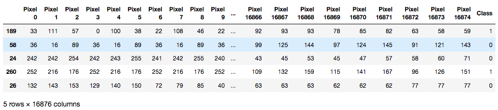
We finally append all breed dataframes together and shuffle the data.

# Combine the pix DF and the Class Df
out_df = pd.concat([data_df, class_df], axis=1)

# Shuffle our dataframe
out_df = shuffle(out_df)

out_df.head()

2) Principal Component Analysis (PCA)

After resizing all image files, we attempted a reduction in the dimensions of our exogenous variables. We noted that a large number of exogenous variables can lead to overfitting and result in high dimensionality to some models. It should also be noted that we have produced exactly 16875 features, while the number of files processed are less than 1000. With this in mind, we reduced the dimension of our dataset using Principal Component Analysis (PCA).

PCA is a way to find the each feature’s variability ratio to overall features variability. It extracts the feature which is the most variable among a given set and is orthogonal to the features already extracted. With the help of PCA, we can extract features that explain a certain level of variability. We used PCA to obtain features which explain more than 90% of the feature set variance. The number of features we gained is 141, which reduced the dimension enormously, compared to the original data of 16875 features.

It should be noted that as the image dimension size increases, so too do the number of features our PCA extracts. This is expected as an image of 100 by 100 pixels should produce close to 30,000 features (significantly larger than our 16,875 features). Our group specifically opted to reduce image dimension size as an effort to reduce the number of inital predictiors.

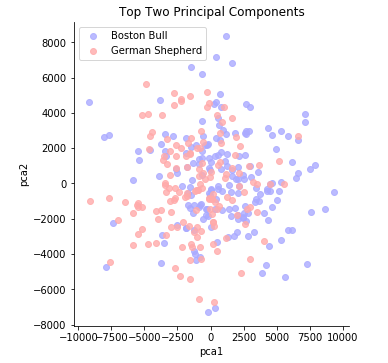
    pca = PCA(n_components=2)
    pca.fit(X_train)
    X_train_pca = pca.transform(X_train)

    X_train_pca_df = pd.DataFrame(X_train_pca, columns=["pca1", "pca2"])
    X_train_pca_df["Class"] = y_train.values
    sns.lmplot(x = "pca1", y = "pca2", hue="Class", data = X_train_pca_df, fit_reg = False, legend = False, palette = 'bwr')
    plt.title("Top Two Principal Components")
    plt.legend();

The first two principal components explain 0.218 of the variance

    pca = PCA()
    X = pca.fit_transform(out_df.drop('Class', axis=1))
    a, num = 0, 0
    for i in range(X.shape[1]):
        a += pca.explained_variance_ratio_[i]
        num += 1
        if a > 0.9:
            break
    pca = PCA(num)
    pca.fit_transform(X)

The first 141 components explain 0.901 of variance

3) Cross-check

After applying PCA to the data set, we split the data into train and test sets, so we can obtain less biased result( i.e. less affected by overfitting phenomenon) by using test set metrics.

    x_train, x_test, y_train, y_test = train_test_split(X, out_df.iloc[:,-1], test_size=0.3)

    y_train = y_train.astype('int')
    y_test = y_test.astype('int')

4) Custom Functions

# Return a beautiful soup object from the provided file
def obtain_annotations (filename):    
    if os.path.exists(filename):
        with open(filename) as fp:
            return BeautifulSoup(fp, "lxml")

# Return the bounding box x,y dimensions for the given image
def obtain_boundBox_loc (soup):
    # Use beautiful soup to parse the label file, ensure our output variables are integer dtypes
    xmin = int(soup.find("xmin").text)
    xmax = int(soup.find("xmax").text)
    ymin = int(soup.find("ymin").text)
    ymax = int(soup.find("ymax").text)
    
    return (xmin, xmax, ymin, ymax)

# Given the dog label, return a enumerated value that corresponds with the dogs breed (0 = bull, 1 = gershep)
def obtain_dogclass (soup):
    breed = soup.find("name").text
    if (breed == 'Boston_bull'):
        return 0
    elif (breed == 'German_shepherd'):
        return 1
    else:
        return None

# Crop the provided image based on the provided bounding dimensions 
def generate_boundBox (img, xmin, xmax, ymin, ymax):
    crop_img = img[ymin:ymax, xmin:xmax]
    return crop_img

# Resize our image to a uniform size and flatten it
# Return a new list containing the raw pixel values
def image_to_feature_vector(image, size):
    return cv2.resize(image, (size, size)).flatten()

def load_images_from_folder(imageFolder, labelFolder, size):
    pixValues = []
    classes = []
    for filename in os.listdir(imageFolder):
        
        img = cv2.imread(os.path.join(imageFolder, filename))
        
        if img is not None:
            
            # Obtain the label information for that picture
            bsObj = obtain_annotations(labelFolder + filename[:-4])
            
            # Obtain the dimensions for the location of the dog
            xmin, xmax, ymin, ymax = obtain_boundBox_loc(bsObj)
            
            # Crop our image such that only the dog is shown
            crop_img = generate_boundBox(img, xmin, xmax, ymin, ymax)
            
            # Obtain a 1D array of every pixel value in the image
            pixValues.append(image_to_feature_vector(crop_img, size))
            
            # Obtain the corresponding enumerated classification value for the dog's breed
            classes.append(obtain_dogclass(bsObj))

    return np.array(pixValues), np.array(classes)

# Appends list values to selected columns given a provided dataframe 
# Returns the update dataframe
def DfAppend_Vals(dataFrame, matrix, columns):
    for vector in matrix:
        dataFrame = dataFrame.append(pd.Series(vector, index = columns), ignore_index=True)

    return dataFrame

2. Dog Breed Classification Models

In the following classification models, we determine success through the comparison of model accuracy scores. In an attempt to improve our model accuracies, we performed hyper-parameters tuning through either the gridsearchcv method, or manually.

1) K-Nearest Neighbors (Varying Image Size)

K-Nearest Neighbors Classification (Knn) classifies data points based on the length-metrics from centroids. In this model, we set two neighbors, Euclidean metrics(by default) and ran the model on multiple unifed image sizes of 25, 50, 75 pixel (identical width by height) dimensions.

Example Image Import without any Bounding Box	Scaled Import Image with a Bounding Box

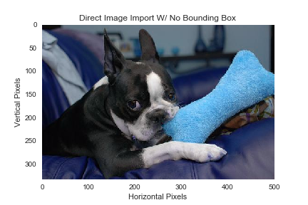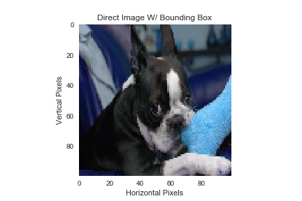The accuracy scores obtained were 0.5445544554455446, 0.4752475247524752, and 0.6237623762376238 respetively. Our impression of these findings, is that as the image dimensions grow in size (thus the more information it contains) conversly produces a higher accuracy score, thus an increase in image size corresponds to an increase in model accuracy. This conclusion is reinforced by the accuracy scores obtained, showcasing that largest image dimensions demonstrated higher accuracy scores than one featuring smallest dimensions.

    nei = knn(2)
    nei.fit(X=x_train, y=y_train)
    y_pred_knn=nei.predict(x_test)
    accuracy_score_size_knn.append(accuracy_score(y_pred_knn, y_test))

Knn accuracy scores of: 0.5445544554455446, 0.4752475247524752, and 0.6237623762376238, using 2 nearest neighbours

3) AdaBoost Classification

AdaBoost Classification classifies data points by correcting previous errors. Multiple classifiers sequentially correct errors and aggregating those gave better results. We used the ‘SAMME” algorithm as we are simply classifying two breeds. The accuracy score we obtained is 0.6039603960396039, 0.6534653465346535, and 0.6138613861386139. It should be noted that our maximum accuracy score achived corresponds to a image sizee of 50 by 50 pixels.

    ada = AdaBoostClassifier(algorithm='SAMME')
    param_grid = {'n_estimators':[10,20,30,40,50,60], 'learning_rate':[0.001, 0.01, 0.1, 1.]}
    gs = GridSearchCV(cv=5, param_grid=param_grid, estimator=ada)
    gs.fit(x_train, y_train)
    cc = gs.best_params_
    ada = AdaBoostClassifier(n_estimators=cc['n_estimators'], learning_rate=cc['learning_rate'])
    ada.fit(x_train, y_train)
    y_p_a = ada.predict(x_train)
    y_pred_adaa = ada.predict_proba(x_train)[:,1]
    y_pred_ada = ada.predict(x_test)
    
    y_pred_adap = ada.predict_proba(x_test)[:,1]
    accuracy_score_size_ada.append(accuracy_score(y_pred_ada, y_test))

AdaBoost accuracy scores of: 0.6039603960396039, 0.6534653465346535, and 0.6138613861386139, using 5-fold cross validation to determine n_estimators from a list of 10, 20, 30, 40, 50, 60

4) Decision Tree Classification

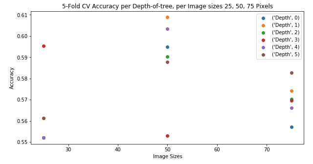
Decision Tree Classification classifies data points based on the splitting principle, where the number of principles is bounded by the max_depth parameter we set (in which we used the argmax value from a range of 1, 3, 5, 7, 10, 15 depths). The accuracy scores obtained were 0.6831683168316832, 0.6237623762376238, and 0.594059405940594 with corresponding image sizes of 25, 50, 75 pixels.

In comparison to our previous Knn results, the accuracy score of decision tree classification decreases as the size of the image file increases. One possible explanation is that our decrease in accuracy is the resulting effect of the number of max_depth parameter utilized, increasing range of depth may aleivitate this issue. Futhermore, while we have a significant amount of information to process, we have only limited splitting principles, and therefore the classification doesn’t use the information we have thoroughly.

    crossVal_scs = []

    for j in range(len(size)): 
    
        C = [1, 3, 5, 7, 10, 15]
        tree_acc = []


        for i in range(len(C)):
            model = DecisionTreeClassifier(max_depth=C[i])
            model.fit(x_train, y_train)
            tree_acc.append(accuracy_score(y_test, model.predict(x_test)))

            scores = cross_val_score(estimator=model, X=x_train, y=y_train, cv=5)
            crossVal_scs.append(scores.mean())

        C_star = C[np.argmax(tree_acc)]
        model = DecisionTreeClassifier(max_depth=C_star)
        model.fit(x_train, y_train)

        y_pred_treet = model.predict_proba(x_train)[:,1]
        y_pred_tree = model.predict(x_test)
        y_pred_treep = model.predict_proba(x_test)[:,1]

        accuracy_score_size_t.append(accuracy_score(y_pred_tree, y_test))

        y_p_t = model.predict(x_train)

crossVal_scs = np.reshape(crossVal_scs, (6, 3))

plt.figure(figsize=(10,5))

for idx, scores in enumerate(crossVal_scs):  
    plt.plot([25, 50, 75], scores, linestyle='None', marker='o', label=("Depth", idx))


plt.title("5-Fold CV Accuracy per Depth-of-tree, per Image sizes 25, 50, 75 Pixels")
plt.xlabel("Image Sizes")
plt.ylabel("Accuracy")
plt.legend()

Decision Tree accuracy scores of: 0.6831683168316832, 0.6237623762376238, and 0.594059405940594, using 5-fold cross validation to determine depth from a depth list of 1, 3, 5, 7, 10, 15

5) Random Forest Classification

Random Forest Classification classifies data points based on the multiple of decision trees. The accuracy scores we received are 0.6831683168316832, 0.6633663366336634, and 0.6039603960396039. We noticed that using a Random Forest classification mode, generally produced better results (when compared against our decision tree classifier), this is agreeable with most of the decision tree classification results. However, since we ran our random forest model based on the tree classifiers, our accuracy scores also decreased as the size increased. We believe the same reasoning behind this issue (model depth accuracy) applies here as well.

    rf = RandomForestClassifier()
    param_grid = {'max_depth':[1,3,5,7,10,15], 'n_estimators':[5,10,15,20,25,30,35],'criterion':['gini', 'entropy']}
    
    gs = GridSearchCV(cv=5, param_grid=param_grid, estimator=rf)
    gs.fit(x_train, y_train)
    cc = gs.best_params_
    
    rf = RandomForestClassifier(max_depth=cc['max_depth'], n_estimators=cc['n_estimators'], criterion=cc['criterion'])
    rf.fit(x_train, y_train)
    
    y_p_r = rf.predict_proba(x_train)[:,1]
    y_pred_for = rf.predict(x_test)
    y_pred_forr = rf.predict_proba(x_train)[:,1]

    y_pred_forp = rf.predict_proba(x_test)[:,1]

    accuracy_score_size_f.append(accuracy_score(y_pred_for, y_test))

Random Forest accuracy scores of: 0.6831683168316832, 0.6633663366336634, and 0.6039603960396039, using 5-fold cross validation to determine depth from a depth list of 1, 3, 5, 7, 10, 15

6) Mixture of Classifiers Classification (Ensembling)

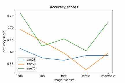
Our final trial performed, utilized a combination of all prior results obtained. We ran a logistic regression model on the probabilities provided by the previous predictions, obtaining a highest score when image size corresponded to the dimension of 25 by 25 pixels. The ensemble model performed relatively well with a uniformed image size of 50 pixels. However, our model did not classifiy well when the image size was increased to a 75 by 75 pixel dimension. We conjectured that this pattern is due to the use of tree classifier, and random forest classifiers based on tree classifier. The worst score was earned by the K-nearest neighbors with size 50.

Overall, the accuracy scores we obtained for this ensembling model were 0.7128712871287128, 0.6831683168316832, and 0.594059405940594 respectively. These results is more or less natural, as we used a decision tree classification and random forest classification, which previously this pattern of decreasing accuracy scores as image size increased.

    train_ = pd.DataFrame(y_pred_treet)
    b_ = pd.DataFrame(y_pred_forr)
    c_ = pd.DataFrame(y_pred_adaa)
    
    train_ = train_.join(b_, how='left', lsuffix='_')
    train_ = train_.join(c_, how='left', lsuffix='_')
    
    test = pd.DataFrame(y_pred_treep)
    b = pd.DataFrame(y_pred_forp)
    c = pd.DataFrame(y_pred_adap)
    
    test = test.join(b,how='left', lsuffix='_')
    test = test.join(c, how='left', lsuffix='_') 
    
    rtcv = LogisticRegressionCV(refit=True)
    rtcv.fit(train_, y_train)
    
    accuracy_score_size_ens.append(accuracy_score(y_test, rtcv.predict(test)))

Ensembled Logistic Regression Meta-model accuracy scores of: 0.7128712871287128, 0.6831683168316832, and 0.594059405940594

3. Conclusion & Future Work

In this report we examined how a suite of classification models could be used to correctly identify between sub-dog breeds. Specifically, our group looked into the comparision of Boston Bulls and German Shepherd breeds. As originally noted, these breeds were chosen based on the basis of their comparatively distinct visual qualities. In aggregating our image dataset for both Boston Bull and German Shepherd images, our team performed a suite of preprocess methods. Addressing noise distortion and irregular image dimensions, we unified our photos through common image dimensionality, cropped using a bounding box algorithm. We finalized our data preparation process by generating a list of pixel features through flattening of each image’s multi-dimensional pixel array.

The predictions garnered from our model classifications varied according to the dimensionality of our images. We noted that our KNN regression model’s accuracy improved as a direct correlation to the dimension growth for our images. Specifically that showcasing larger image dimensions demonstrated higher accuracy scores than images featuring smaller unified dimensions. While we initially expected this relationship to be mainted across our remaining models, we found instead that our Decision Tree Classification, Random Forest Classification and Logistic Regression meta models performed in contrary to this expecation. We deduced that this was a possible result of insufficient depth range, or likely an issue with predictor size verus observasion count (such that the latter was smaller than the former).

Our group recognizes that our models suffer from innacuracy due to having more observations than predictors. We believe that future inclusion of a Least Absolute Shrinkage and Selection Operator (LASSO) regression could aleiviate this issue, and provide improved model accuracy.

In addition, we need to expand our classification of sub-breeds to include a wider diversity of dog breeds. Our models classified breeds with visual distinct qualities, future work could approach how similar dog breeds can be classified, not only on breed colour, but geometric facial features using a Scale-Invariant Feature Transform (SIFT) algorithm.